Reinforcement Learning with Atari River Raid

Atari games have become a test piece for new RL methods, in part due to the publication of “Human-level control through deep reinforcement learning”. Such games provide a challenging domain that is relatively easy to implement and also relatively easy to understand.

This blog post focuses on finding a reinforcement learning solution to the Atari game River Raid, which is vertically scrolling shooter game developed by Activision in 1982. The player pilots a fighter jet over a river to conduct a raid behind enemy lines. The player can maneuver left or right, accelerate or decelerate, and fire. Points are scored for every enemy shot down. The jet refuels when it flies over fuel depots (fuel depots can also be shot to gain points). The game ends when the fighter jet crashes into the river bank or an enemy craft, or runs out fuel. The fuel gauge is displayed at the bottom of the screen.

Previous Work

In this blog post I replicate the seminal work by Mnih et. al [2015] which developed the deep Q-network bridging the divide between high-dimensional sensory data (eg 210x160 pixel Atari screen) and actions taken by an agent. They achieved this by using a convolutional neural network to map from the high-dimensional Atari input screen to the long-term discounted value for each possible action. Previously, training such a neural network was highly unstable or computationally too expensive to do on a large convolutional network. The key to properly training the neural network was in using two key concepts – experience replay and periodic updates via a target network. With these concepts, they achieved high performance across a set of 49 Atari games.

Experience replay is a biologically inspired phenomenon that shuffles the data being fed to NN for back propagation. In this way, correlations created by sequential feeding data to the NN can be removed. Experience replay can also help to smooth over changes in the state-action-reward history.

The second key method, periodic updating of a target network, helps to decouple the action-value pairs from the target network itself. In calculating Q(s,a) we use the next state Q(s’, a’). The states s and s’ will likely look very similar since they are only one step apart and hence it will be difficult for the neural network to distinguish them. So, by updating the NN at every step, Q(s,a) will influence our value for Q(s’,a’) and other similar states inadvertently and hence introduce instability to the training process. To prevent this the target network is only updated every n steps (where eg n = 1000).

One more quick note before we jump into the code. There is an excellent implementation of this algorithm for Atari Pong given in Deep Reinforcement Learning Hands-On chapter 6 by Maxim Lapan. The source code can be found here. My implementation follows a similar outline.

Image Preprocessing

To decrease the time required to train the model and increase the model’s accuracy, several preprocessing steps are executed. The preprocessing steps are executed in the wrappers.py file and connected in the pipeline function as shown below:

def pipeline(env_name):
    env = gym.make(env_name)
    env = FireOnReset(env)
    env = ResetOnEndLife(env)
    env = SkipFrames(env, 4)
    env = GrayScale(env)
    env = Crop(env, [2,163,8,160])
    env = Dilate(env)
    env = Compress(env)
    env = Buffer(env)
    env = Normalize(env)
    return env

I’ll quickly walk through the purpose of each function (the code for each function can be found in the github repo at the bottom of the page).

• FireOnReset is used to push the fire button which starts the game. This helps speed up training and convergence as the Agent can become stuck at this position for many frames without firing. .ResetOnEndLife is used to split the game at each new life. The game starts with 3 lives.
• SkipFrames is used to speed up training. The difference between one frame and then next is very small and a stable NN will likely choose the same action. To speed training, the Agent selects an action and the action is repeated for n steps (n = 4 in this case).
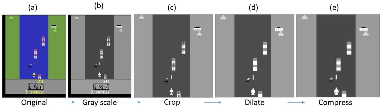
• GrayScale (not GOT) is used to convert the RGB image input to a single channel gray scale image.
• Crop is used to crop the image down to the provided indices.
• Dilate is used to perform image dilation. This is very help in the case where objects on the Atari screen are too small relative to the size of the convolutional filter kernels.
• Compress is used to compress the image to 84x84.
• Normalize is used to renormalize the data from 0-256 to 0.0-1.0.

Figure 1. shows (a) the unprocessed input image from Atari River Raid and (b)-(e) the processed image after passing through each step of the pipeline function.

The deep Q network is defined identical to what was used by Mnih et. al. The input is a 84x84 image as shown below in Figure 1(b). This input image is fed through a 3 layer convolution neural network followed by two fully connected layers. The first convolution layer takes the single channel input image and produces 32 channels with a kernel size of 8 and stride of 4. The next convolutional layer takes the 32 channel input and outputs 64 channels after processing with a kernel of size 4 and stride 2. The final convolutional layer takes the 64 channel input and outputs 64 channels after processing with a kernel size of 3 and stride of 1. The neural network definition is similar to that used by [2].

class DQN(nn.Module):
    def __init__(self, input_shape, n_actions):
        super(DQN, self).__init__()
        self.conv = nn.Sequential(
            nn.Conv2d(input_shape[0], 32, kernel_size=8, stride=4),
            nn.ReLU(),
            nn.Conv2d(32, 64, kernel_size=4, stride=2),
            nn.ReLU(),
            nn.Conv2d(64, 64, kernel_size=3, stride=1),
            nn.ReLU()
        )
        conv_out_size = self._get_conv_out(input_shape)
        self.fc = nn.Sequential(
            nn.Linear(conv_out_size, 512),
            nn.ReLU(),
            nn.Linear(512, n_actions)
        )
    def _get_conv_out(self, shape):
        out = self.conv(torch.zeros(1, *shape))
        return int(np.prod(out.size()))
    def forward(self, x):
        conv_out = self.conv(x).view(x.size()[0], -1)
        return self.fc(conv_out)

The Agent is implemented in model.py and uses the epsilon-greedy approach to determine actions at any given step. The Agent is responsible for taking actions and appending the results to the experience buffer.

class Agent:
    def __init__(self, env, exp_buffer):
        self.env = env
        self.exp_buffer = exp_buffer
        self._reset()
    def _reset(self):
        self.state = self.env.reset()
        self.total_rewards = 0.0
    def play_step(self, net, epsilon=0.0, device="cpu"):
        done_reward = None
        if np.random.random() <  epsilon:
            action = self.env.action_space.sample()
        else:
            state_v = torch.tensor(np.expand_dims(self.state, axis=0)).to(device)
            q_vals_v = net(state_v)
            action = int(torch.max(q_vals_v, dim=1)[1])
        new_state, reward, is_done, info = self.env.step(action)
        self.total_rewards += reward
        self.exp_buffer.append([self.state, action, reward, is_done, new_state])
        self.state = new_state
        if is_done:
            done_reward = self.total_rewards
            self._reset()
        return done_reward

The training is executed in the main.py file which can be found in repository for the project. This file also contains methods to collect and plot the models progress. The model was trained using an Nvidia GeForce GTX 970. The smoothed reward as a function of frames observed is shown in Fig. 2 below.

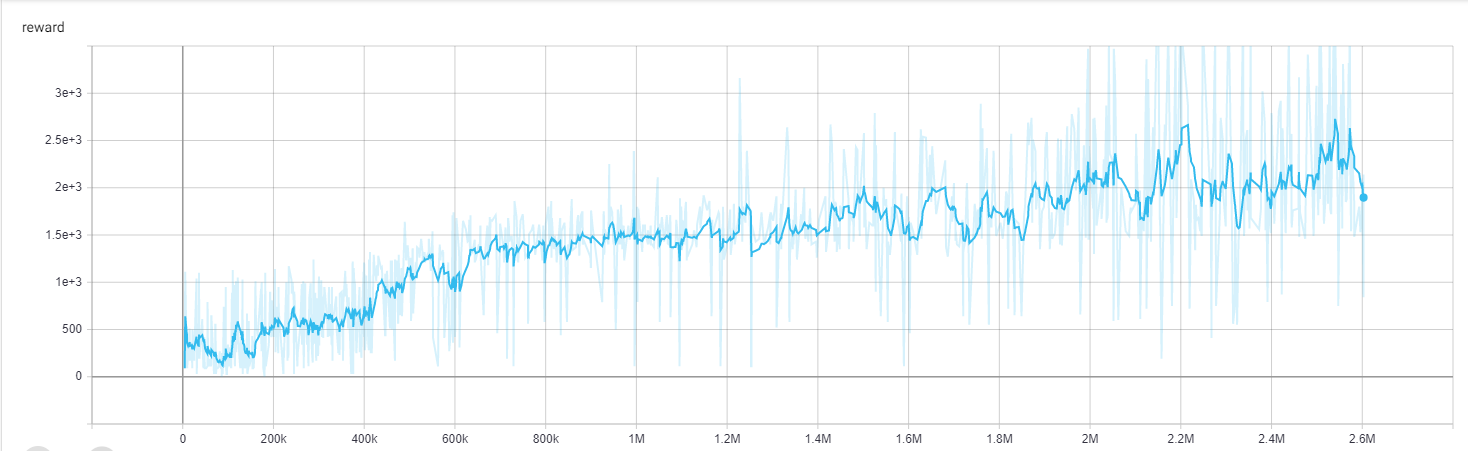
The model appears to learn fairly quickly from ~400k to 700k and then begins to saturate after ~2 million frames observed. In addition, the variablity in acheived score (shown in light blue) appears to increase substaintially with increasing number of frames observed. The video below shows the sixteen epsiodes played by the final state of the model with an epislon of 0.03. This epsilon was chosen to simulate randomness since the Atari games are all deterministic. Such a low value of epsilon shouldn’t have an appreciable impact on the total reward.

After about five rounds of river raid I was able to achieve a score similar to the maximum score observed from the model. The performance reported by Mnih et. al was ~8316 using all three lives. This score is slightly better than the score of ~6800 (across three lives) achieved in this report. The score of an expert player is reported by Mnih et al. to be ~13513. The difference in score between my agent and the one reported by Mnih et al. could be due to the fact that they rescaled the score to range from -1, 1 whereas I’m using the original score reported given by Atari. It could also be due to the length of time the models were allowed to train.

Future Areas to Explore

Watching the model train several times, I’ve noticed that the game seems to have trouble getting past certain points in the game. For example, when the agent encounters it’s first bridge or when the agent encounters a constriction in the river. These difficult points can be visualizzed by looking at the distribution of scores for a single life episode on the trained agent. This distribution is shown below in Fig. 4.

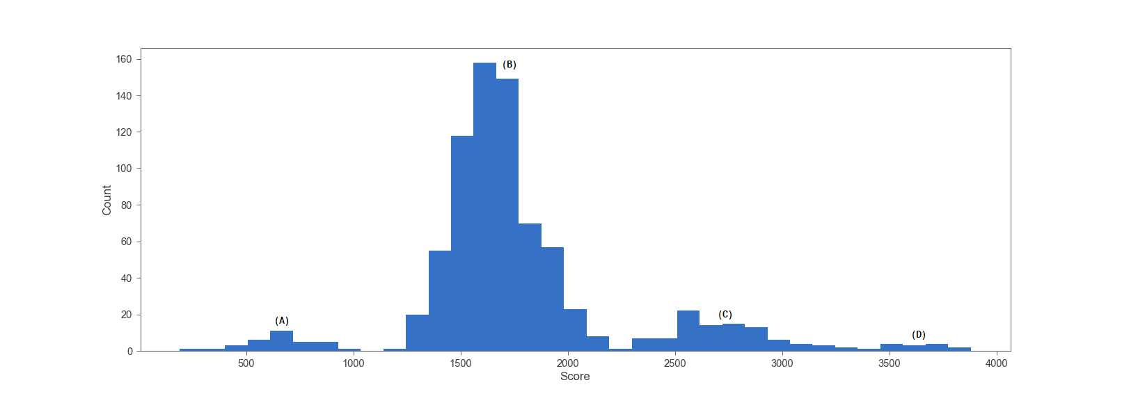
Figure 4 shows 4 clear distributions labeled (a)-(d). Distribution (a) seems to correspond to the death before the first bridge by one of the small helicopters (likely hard for the agent to see in the compressed image). Distribution (B) seems to correspond to making it past the first bridge and past the first split in the river, but dying before the second bridge. Distribution (C) seems to have made it past the second bridge, but died before the third. Finally, distribution (D) has made it past the third bridge, but usually dies by running out of fuel.

It would make sense if there were a way to more greatly weight or increase the importance of how the agent died. This might allow the agent to focus more on its weaknesses and hence improve training speed. One simple method for achieving this is select the images from the replay buffer acording to some probability distribution describing the importance of each training snap shot.

References

[1] Mnih, V., Kavukcuoglu, K., Silver, D. et al. Human-level control through deep reinforcement learning. Nature 518, 529–533 (2015). https://doi.org/10.1038/nature14236

[2] Maxam Lapan, Deep Reinforcement Learning Hands-On: Apply modern RL methods, with deep Q-networks, value iteration, policy gradients, TRPO, AlphaGo Zero and more. Packt Publishing, Ch. 6 (2018).

[3] https://github.com/joseywallace