Neural networks from scratch

In this post I go through the mathematics behind neural networks and demonstrate how to implement a neural network in python from scratch. First, I’ll introduce the simple example of a single neuron with a sigmoid activation function. The neuron is the fundamental unit from which neural networks are designed. The single neuron model is used to introduce the concepts of gradient descent and back propagation before applying these concepts to the more complicated neural network.

The perceptron, which was the precursor to the sigmoid neuron was invented by Frank Rosenblatt in the 1950s and 60s. The concept of the perceptron, which is biologically inspired, takes the sum of multiple weighted inputs and compares this sum to some threshold value. If the value is greater than the threshold, the neuron ‘fires’ creating an output of unity. Otherwise, the neuron outputs zero. Neurons can be programmed by adjusting their weights and biases, to simulate ‘and’, ‘or’, and ‘nand’ gates. Multiple neurons can be strung together to form literally any logic circuit imaginable. If we can then string multiple of these neurons together in layers and somehow optimize the system towards a particular solution to a problem, then we have an algorithm for designing complex possibly non-intuitive circuits that given some input can produce the desired output. That’s a huge if.. It’s truly amazing that such a technique exist. The two key components that make up this optimization technique are back propagation and stochastic gradient descent. Both are actually fairly simple to understand requiring only an understanding of basic calculus. Gradient defines the method by which we seek to minimize the cost function and hence the error in our model. Back propagation is a technique for optimizing the influence of a each weight and biases on the cost function.

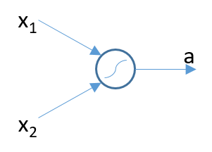
The figure below shows the simple single neuron model with two inputs and a single output.

It is useful to define z as shown below:

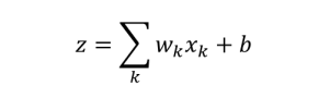
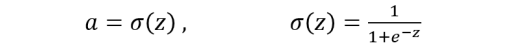
Where w_k are the weights, x_k are the input values, and b is the bias. The z function, known as the weighted input to the neuron, is passed through a non-linearity function in this example a sigmoid. The sigmoid function allows us to optimize the weights and biases much more easily since as opposed to the perceptron model discussed above, the sigmoid is continuous. In addition the derivative of the sigmoid is simply σ = σ(1-σ). The final output of the neuron, a, is shown below along with the σ function.

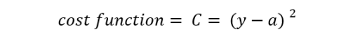
The cost function can be defined as the square of the difference between a and the true value y as shown below:

As discussed above, our approach to optimize this neuron is to find the gradient of the cost function with respect to the weights and bias and step in the opposite direction of this gradient. The gradient is derived via the chain rule as shown below:

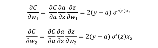
Once we have found the gradient, we want to step in the opposite direction of the gradient by some step size which is defined by the learning rate η.

Let’s put this all together in python now. The Neuron class shown below is initialized by passing in the number of epochs (training steps over the entire dataset), eta (learning rate), and dim (length of input vector X).

import numpy as np
class Neuron:
    def __init__(self, dim, epochs, eta):
        self.epochs = epochs
        self.eta = eta
        self.w = np.array([0.1]*dim)
    def fit(self, x, y):
        for i in range(self.epochs):
            del_w =  del_b = 0
            for xt, yt in zip(x,y):
                z = self.w[0] + self.w[1:].dot(xt)
                sigz = self.sigma(z)
                delC = 2*(yt - sigz)*sigz*(1-sigz)
                del_w += delC*xt
                del_b += delC
            self.w[0] += (self.eta/len(x))*del_b
            self.w[1:] += (self.eta/len(x))*del_w
    def sigma(self, z):
        return 1/(1+np.exp(-z))

The single neuron acts as a linear separator and hence we can test the Neuron class on the data set created below:

x = 2*np.random.rand(100,2) - 1
y = x.dot((1,-1.5)) > 0.4

n = Neuron(2, 1500, 1)
n.fit(x,y)

plt.scatter(x[:,0], x[:,1], c=y)
z = x.dot(n.w[1:]) + w[0]
plt.scatter(x[:,0], x[:,1], c=n.sigma(z))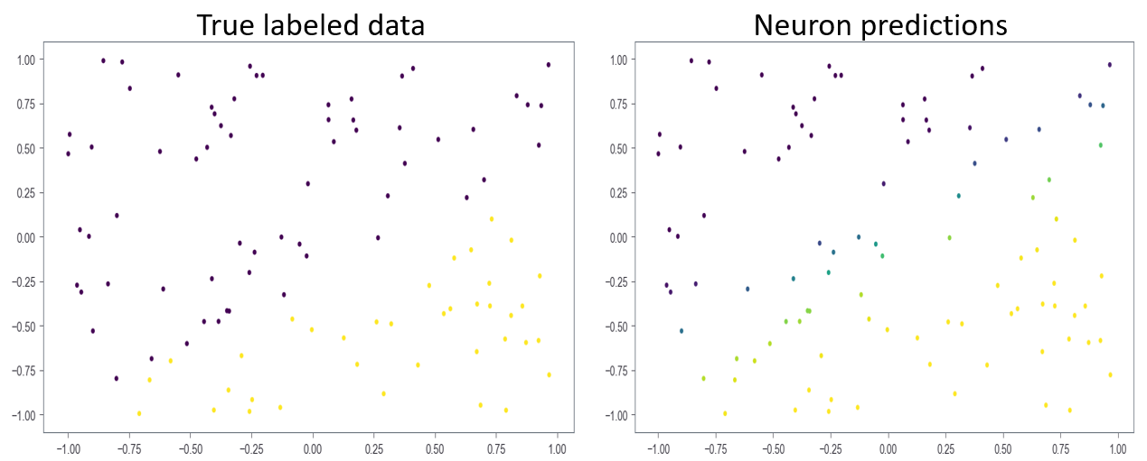

As shown in Figure 2 above, the single neuron does a decent job of separating the data. If the data is not linearly separable, the neuron will not find an optimal solution. In this case, at least one hidden layer is required.

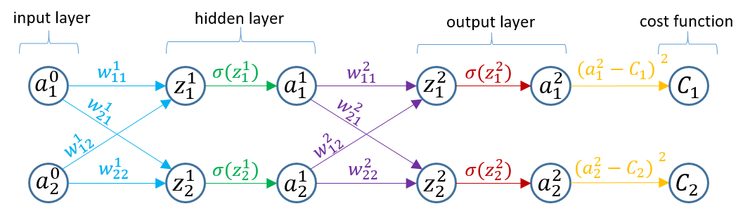
Now that we have had a quick refresher on the concepts of gradient descent and back propagation on a simple single neuron model, let’s move to the more complex model shown below.

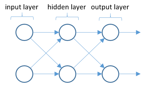
This neural network is composed of a two neuron input layer, followed by a single two neuron hidden layer and finally, a two neuron output layer. I think this network is the simplest network were we can still get an idea of how to handle the multidimensional weight matrices and gradients. In the figure below, I have expanded the network to include a node for each operation. z nodes represent nodes in which the summation operation occurs, a nodes apply the nonlinearity function in this case a sigmoid, and C nodes apply the cost function.

Weights for each connection are show in the figure. Note that the super script denotes the level within the neural network and the subscript, ij, denotes that the weight is going from node j to node i. It is indexed this way to keep consistency with the weight matrix as you will see shortly.

With the neural network outlined as shown in Fig. 4, each connection represents a partial derivative, which when strung together make up the chain rule. For example, if you want to know the derivative of the cost function with respect to the weight w11, you start at node C1 and find the product of partial derivatives of the child node with respect to the parent node until you reach the node of interest. This process is shown below for the weights and biases at level L=2 in the network. Note that each derivative is color coded to match Fig. 4.

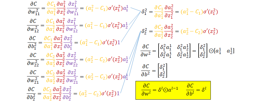
The δ terms defined in the right column of equations above are seen to repeat in all terms. Looking more closely we see that these δ terms are actually the error propagated backwards from through the cost and sigmoid functions. In other words, δ² is the vector of errors associated with the l^th level of the neural network. The gradient of the cost function with respect to the weights can be condensed into a matrix form as shown above in the right columns of equations, where ⨀ represents the Hadamard product of the two matrices. In addition, the gradient of the cost function with respect to the bias is simply δ.

The equations for the gradient of the cost function with respect to weights in level 1 of the neural network are shown below.

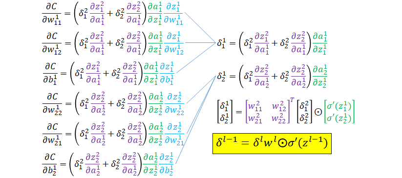
The main difference compared to gradient at level L=2 in the neural network is in that the weights can affect the cost function through two separate branches. Similar to the previous layer, we can define δ¹ (right column) for level L=1. δ² is defined in terms of δ² and hence can be rewritten as shown in the highlighted box above. This equation along with the other two in highlighted equations above make up the general approach for calculating the weights and biases iteratively starting at the output layer and moving back towards the input. These are the primary equations we will use in implementing the back propagation code.

Now that we have derived the primary equations for back propagating the error through the network, let’s move on to the code. First, we will define the NeuralNet class init and feed forward:

import numpy as np
class NeuralNet:
    def __init__(self, sizes):
        self.w = [np.random.rand(sizes[i], sizes[i-1]) for i in range(1,len(sizes))]
        self.b = [np.random.rand(sizes[i], 1) for i in range(1, len(sizes))]
        self.n = len(sizes)
    def feed_forward(self, x):
        a = x
        for w, b in zip(self.w, self.b):
            a = self.sigmoid(np.matmul(w, a) + b)
        return a

In the init method, the weights and biases are defined as a lsit of numpy arrays, where the list index +1 represents the layer.

The optimization technique can be broken up into the following task:

1. Partition the data into minibatches
2. Calculate the gradient of the cost function via back propagation
3. Calculate the step based on learning rate and gradient
4. Apply a step change to weights and biases
5. Rinse and repeat for each minibatch for n epochs

We can break this into two functions (1) stochastic gradient descent (sgd) and (2) backpropagation. The sgd method is responsible for all of the above steps except 3, which the back propagation method handles. The code for the sgd method is shown below. The method loops over though the data epochs number of times, shuffling the data and creating new minibatches at each epoch. Then, the code loops through each minibatch and each instance within each minibatch creating three nested for loops. The runtime is O(epochs*len(x)).

    def sgd(self, x, y, epochs, eta, batch_size, x_test=None, y_test=None):
        for j in range(epochs):
            idx = np.random.permutation(x.shape[0])
            xr, yr = x[idx], y[idx]
            minibatches = [(xr[k:k+batch_size], yr[k:k+batch_size])
                        for k in range(0, xr.shape[0], batch_size)]
            for xm, ym in minibatches:
                grad_w = [np.zeros(w.shape) for w in self.w]
                grad_b = [np.zeros(b.shape) for b in self.b]
                for xi, yi in zip(xm, ym):
                    d_grad_w, d_grad_b = self.backpropagate(xi, yi)
                    grad_w = [dw+w for dw, w in zip(d_grad_w, grad_w)]
                    grad_b = [db+b for db, b in zip(d_grad_b, grad_b)]
                self.w = [w-eta*(dw/xm.shape[0]) for w, dw in zip(self.w, grad_w)]
                self.b = [b-eta*(db/xm.shape[0]) for b, db in zip(self.b, grad_b)]
            if x_test and y_test:
                print('Epoch:', j, 'Score:', self.score(x_test, y_test), '%')

The next function is backpropagation. This function first takes in a single training instance and returns the weight and bias gradients for that instance. First, the function performs a forward pass through the network, collecting the z and a values along the way. Then, the δ, w, and b are calculated for the last layer in the network (this layer is calculated differently than the rest of the layers due to the cost function). Next, the δ, w, and b for each subsequent layer working back towards the input of the neural network are calculated using an iterative dynamic programming approach. Finally, the resulting gradient of w and b is returned.

    def backpropagate(self, x, y):
        grad_w = [np.zeros(w.shape) for w in self.w]
        grad_b = [np.zeros(b.shape) for b in self.b]
        #forward pass to calculate the 'z' and 'a' values
        a_vals, z_vals = [x], []
        for w, b in zip(self.w, self.b):
            z_vals += [np.matmul(w, a_vals[-1]) + b]
            a_vals += [sigmoid(z_vals[-1])]
        #backward pass propagating errors through the network
        delta = (a_vals[-1] - y)*sig_prime(z_vals[-1])
        grad_w[-1] = delta.reshape(-1,1)*a_vals[-2]
        grad_b[-1] = delta
        for l in range(2, self.n):
            delta = np.matmul(self.w[-l+1].T, delta)*sig_prime(z_vals[-l])
            grad_w[-l] = delta.reshape(-1,1)*a_vals[-l-1]
            grad_b[-l] = delta
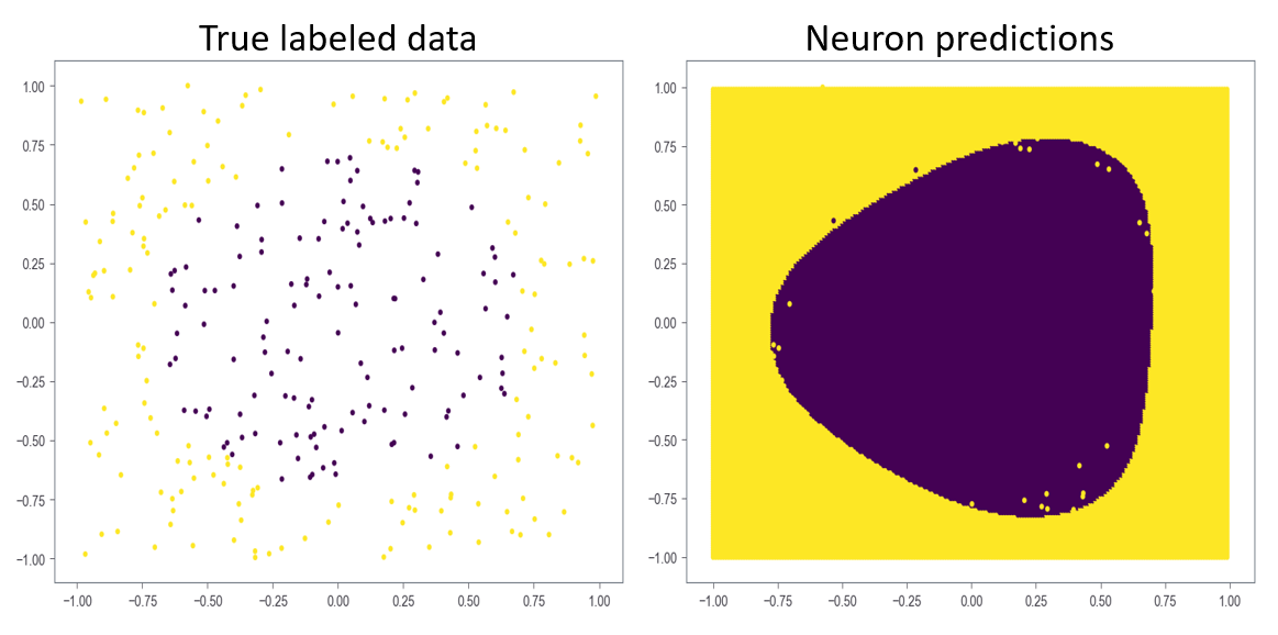
        return grad_w, grad_b 

As a quick validation, we can test a neural networks ability to fit non-linearly-separable data. Figure 5 below shows the result of fitting a neural network with sizes = (2,3,2) to a data set where all labels within a given radius are classified as 1 and all outside the radius are classified as 0.

Resources and Additional Reading

[1] Neural networks and Deep Learning by Michael Nielsen, Dec. 2019

[2] 3Blue1Brown youtube series on neural networks

[3] Code repository for this blog post