Image Stabilization Via Gaussian Filters in OpenCV
Stabilizing shaky video via parametric image alignment and Guassian smoothing

This tutorial demonstrates the process of image stabilization in python using the OpenCV library. The code for this demonstration, including several helper functions used to plot and visualize the transformation can be found on my github page below. The image stabilizaation pipeline involves three main steps – (1) determining the original path of the camera, (2) smoothing this path, and (3) applying the smoothed path to the image set.
Finding the Camera’s Path
The camera’s path can be determined by finding the warp matrix from one image to the next in the series. This matrix allows us to transform or map from one camera coordinate system to another. The first step in determining this matrix, is deciding on a suitable model for the geometric transformation from one frame to the next. The most common choices are either affine or pure translation, however, other methods rely on projective transformation (homography) or even non-linear transformations. In this tutorial, we will assume Euclidean motion and use the following transformation:

Where, (x, y) and (x’, y’) are the pixel coordinates in the original and stabilized system, respectively. The vector (Tx, Ty) represents the camera’s translation and θ is the camera’s rotation, both relative to some initial reference frame. The second equation uses the homogeneous form which brings the translation and rotation terms into a single matrix. This matrix is known as the warp matrix, since it can be used to warp an image from one coordinate frame to another.
Determining the warp marp matrix
There are several methods for determining the warp matrix. All methods involve looking for some type of correspondence between two images. These correspondences can be either sparse (ie feature matching between images with RANSAC) or dense (Lucas-Kanade optical flow). Both of these methods can be computationaly intensive for longer videos. A more recent method that runs faster (in some cases) and is more stable (in some cases) is the so-called “Parametric Image Alignment using Enhanced Correlation Coefficient Maximization”[1]. This method uses an “enhanced” correlation coefficient for the similarity metric that is robust against geometric and photometric distortions. In addition, the iterative approach the authors use linearizes the problem making it much faster than directly solving the non-linear objective function. This method can be employed in OpenCV via the findTransfromECC function as shown below.
def get_warp(img1, img2, motion = cv2.MOTION_EUCLIDEAN):
    imga = img1.copy().astype(np.float32)
    imgb = img2.copy().astype(np.float32)
    if len(imga.shape) == 3:
        imga = cv2.cvtColor(imga, cv2.COLOR_BGR2GRAY)
    if len(imgb.shape) == 3:
        imgb = cv2.cvtColor(imgb, cv2.COLOR_BGR2GRAY)
    if motion == cv2.MOTION_HOMOGRAPHY:
        warpMatrix=np.eye(3, 3, dtype=np.float32)
    else:
        warpMatrix=np.eye(2, 3, dtype=np.float32)
    warp_matrix = cv2.findTransformECC(templateImage=imga,inputImage=imgb,
                                       warpMatrix=warpMatrix, motionType=motion)[1]
    return warp_matrix

def create_warp_stack(imgs):
    warp_stack = []
    for i, img in enumerate(imgs[:-1]):
        warp_stack += [get_warp(img, imgs[i+1])]
    return np.array(warp_stack)
The get_warp function takes as input the two images and the motion model (Euclidean in this example) to be used and returns the warp matrix. The create_warp_stack simply calls the get_warp on a list of images and returns the 3D numpy array of warp matrices. It is important to note the warp matrices are between neighboring pairs of images. As a result, the homography matrices represent the change in motion between the frames. We could think of these delta values as the derivative of position with respect to the frame number (or a velocity of sorts). The trajectory can be determined from integrating over the velocity via a product of warp matrices:
Where H is the warp matrix. The function below yields the nth integrated warp matrix on the nth call.
def homography_gen(warp_stack):
    H_tot = np.eye(3)
    wsp = np.dstack([warp_stack[:,0,:], warp_stack[:,1,:], np.array([[0,0,1]]*warp_stack.shape[0])])
    for i in range(len(warp_stack)):
        H_tot = np.matmul(wsp[i].T, H_tot)
        yield np.linalg.inv(H_tot)
These three function represent the first step in the image stabilization pipline. Now, let’s try applying these functions to some video. The video below was taken while moving the camera in both panning motions and shaky random motions.
Finding camera the velocity and trajectory
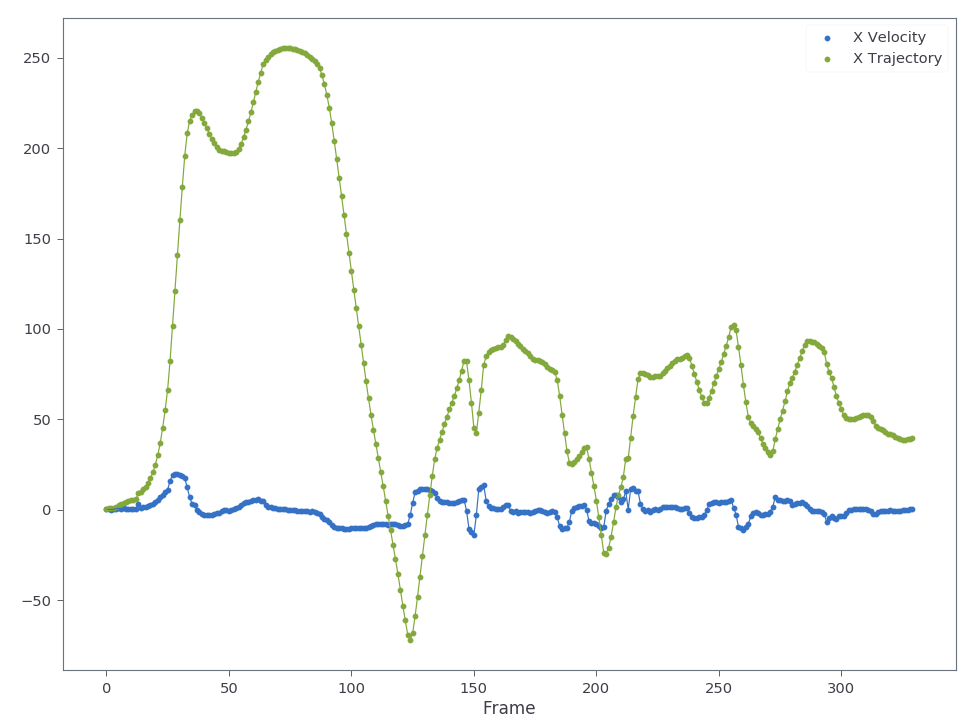
We can run the create_warp_stack method to find the camera’s motion through the video and plot the velocity and trajectory as shown below. The trajectory is found by doing a cumulative summation over the warp stack.
ws = create_warp_stack(imgs)
i,j = 0,2
plt.scatter(np.arange(len(ws)), ws[:,i,j], label='X Velocity')
plt.plot(np.arange(len(ws)), ws[:,i,j])
plt.scatter(np.arange(len(ws)), np.cumsum(ws[:,i,j], axis=0), label='X Trajectory')
plt.plot(np.arange(len(ws)), np.cumsum(ws[:,i,j], axis=0))
plt.legend()
plt.xlabel('Frame')
Visualizing the motion by stablizing the camera
We can visualize this motion by applying the warp stack to each image in the sequence via OpenCV’s warpPerspective function. This function applies the warp matrix to each of the source image pixel’s x,y location to determine it’s coordinates in the warped image. Care must be taken to ensure the images are not pushed outside the display bounds. The function give below solves this problem adding a translation offset to the warp matrix and another offset to the openCV warpPerspective function. These offsets are determined from finding the maximum and minimum coordinates for the image corners. The helper function used to find these values is given in the appendix.
def apply_warping_fullview(images, warp_stack, PATH=None):
    top, bottom, left, right = get_border_pads(img_shape=images[0].shape, warp_stack=warp_stack)
    H = homography_gen(warp_stack)
    imgs = []
    for i, img in enumerate(images[1:]):
        H_tot = next(H)+np.array([[0,0,left],[0,0,top],[0,0,0]])
        img_warp=cv2.warpPerspective(img,H_tot,(img.shape[1]+left+right,img.shape[0]+top+bottom))
        if not PATH is None:
            filename = PATH + "".join([str(0)]*(3-len(str(i)))) + str(i) +'.png'
            cv2.imwrite(filename, img_warp)
        imgs += [img_warp]
    return imgs
The resulting video as well as the x trajectory are shown in the figure below.
This video in Fig. 3 shows a fully stabilized warp of the original shaky video. You might notice there are some artifacts after the warp. When the camera pans very quickly you get an effect known as the “rolling shutter effect”. The effect occurs due to the fact that the image sensor continues to gather light during the acquistion process. The camera pixels are read sequentially from top to bottom or right to left. Thus, one side of the camera sees a slightly different image than the other side. This creates the “wobble” or “jello-like effect” seen above.
Determining the smoothed camera trajectory
Although the video in Fig.3 was interesting to make, we ideally don’t want to see any black regions around opur final product. Cropping is one obvious solution. However, with this much motion, there is no reasonably sized window that could eliminate all black regions. There are two options – (1) motion inpainting or (2) smoothing the trajectory. The first option involves using information from previous/future frames to guess what should be outside the range of the current frame and “inpainting” those pixels. The second approach involves trying to estimate the intended motion the camera-person wanted and removing the high frequency surrounding that signal. The second approach involves separating the camera’s intended path from the high frequency instabilities. This post focuses on the second approach using a simple gaussian filter to remove the high frequency noise.
In order to compute the smoothed trajectory, we need the original trajectory, averaging window size, and sigma for the smoothing gaussian. The gauss_convolve function below takes these as input and returns the smoothed trajectory as shown below. Since we must smooth all components in the warp matrix stack, it is easiest to pass the sigma values for each element of the warp matrix as a matrix itself. The second function, moving_average, shown below takes the warp stack and sigma matrix as input and calls the gauss_convolve function on each element in the warp matrix. After finding the new trajectory, a derivative kernel is applied ([0,1,-1]) in order to get the velocity which is what the warp matrix is represented by.
def gauss_convolve(trajectory, window, sigma):
    kernel = signal.gaussian(window, std=sigma)
    kernel = kernel/np.sum(kernel)
    return convolve(trajectory, kernel, mode='reflect')

def moving_average(warp_stack, sigma_mat):
    x,y = warp_stack.shape[1:]
    original_trajectory = np.cumsum(warp_stack, axis=0)
    smoothed_trajectory = np.zeros(original_trajectory.shape)
    for i in range(x):
        for j in range(y):
            kernel = signal.gaussian(10000, sigma_mat[i,j])
            kernel = kernel/np.sum(kernel)
            smoothed_trajectory[:,i,j] = convolve(original_trajectory[:,i,j], kernel, mode='reflect')
    smoothed_warp = np.apply_along_axis(lambda m:
                     convolve(m, [0,1,-1], mode='reflect'), axis=0, arr=smoothed_trajectory)
    return smoothed_warp, smoothed_trajectory, original_trajectory
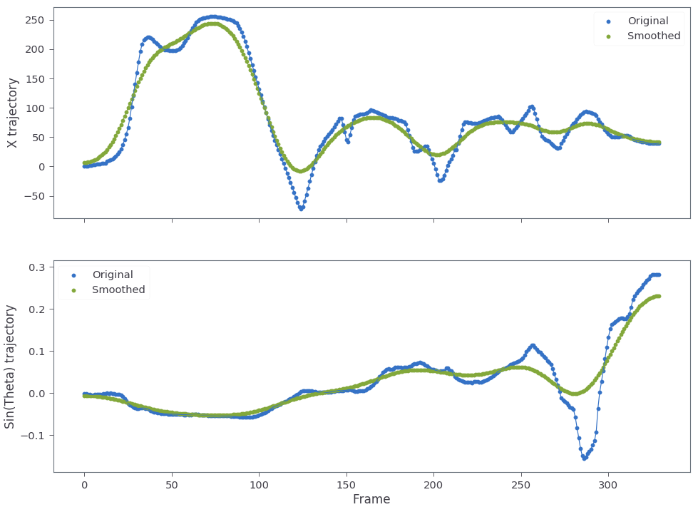
Applying moving_average to the warp matrix stack with a sigma matrix given by:
gives a somewhat weak smoothing in x and y and stronger smoothing for rotation. The resulting trajectory for X and theta is shown below.
This smoothing can be applied as to the images as follows:
warp_stack = create_warp_stack(imgs)
smoothed_warp, smoothed_trajectory, original_trajectory = moving_average(warp_stack,
    sigma_mat= np.array([[1000,15, 10],[15,1000, 10]]))
new_imgs = apply_warping_fullview(images=imgs, warp_stack=warp_stack-smoothed_warp, PATH='./out/')
Note that the warp matrix stack fed to the apply_warping_fullview is not simply the smoothed_warp, but instead the difference of the original warp stack and the smoothed warp stack. This is because the smoothed_warp represents the part of the motion we want to keep, whereas the difference is only the high frequency components. The resulting video after applying the new warp stack is shown below:
Applying the new warp allows the camera to pan left and right without moving significantly outside the original image area. The main contributor to the somehwat large black boundaries are now the rotation terms. Decreasing the rotation sigma values could further reduce the black boundaries (ie increase the final cropped image size).
A good image stabilization algorithm should be fairly stable against salient points in the image (ie someone walking into and out of the camera’s frame). The two video’s below test the image stabilization algorithm against salient points. In both these videos I’m running while filming. The first video is taken parallel with the direction I’m running whereas the second example the camera is ~30 degrees to my direction.
In both cases I reused the same sigma matrix as used above in Fig. 5. Both videos appear quite stable against salient image points. From these examples we can see that the gaussian kernel smoothing is quite effective at stabilizing images. However, compared to the state-of-the-art image stabilization work done by google[2-3], these stabilization techniques are still quite primitive. Google’s algorithm actually uses cinamatography principles to determine the ideal path. They assume that the desired path should be composed of constant, linear, and parabolic segments only. This methodology eliminates unwanted camera drift and that a simple gaussian convolution would not remove. More on this technique to come!
References
[3] Google AI Blog: Auto-Directed Video Stabilization with Robust L1 Optimal Camera Paths”
[4] Learn OpenCV: Video Stabilization Using Point Feature Matching in OpenCV
[5] Github code for this blog post
Note: This code was originally written in partial fulfillment of Georgia Tech’s CS6475 (Computational Photography).