Calculating cascade density using TRIM, OVITO, and python
Method used in the paper: Deterministic Role of Collision Cascade Density in Radiation Defect Dynamics in Si
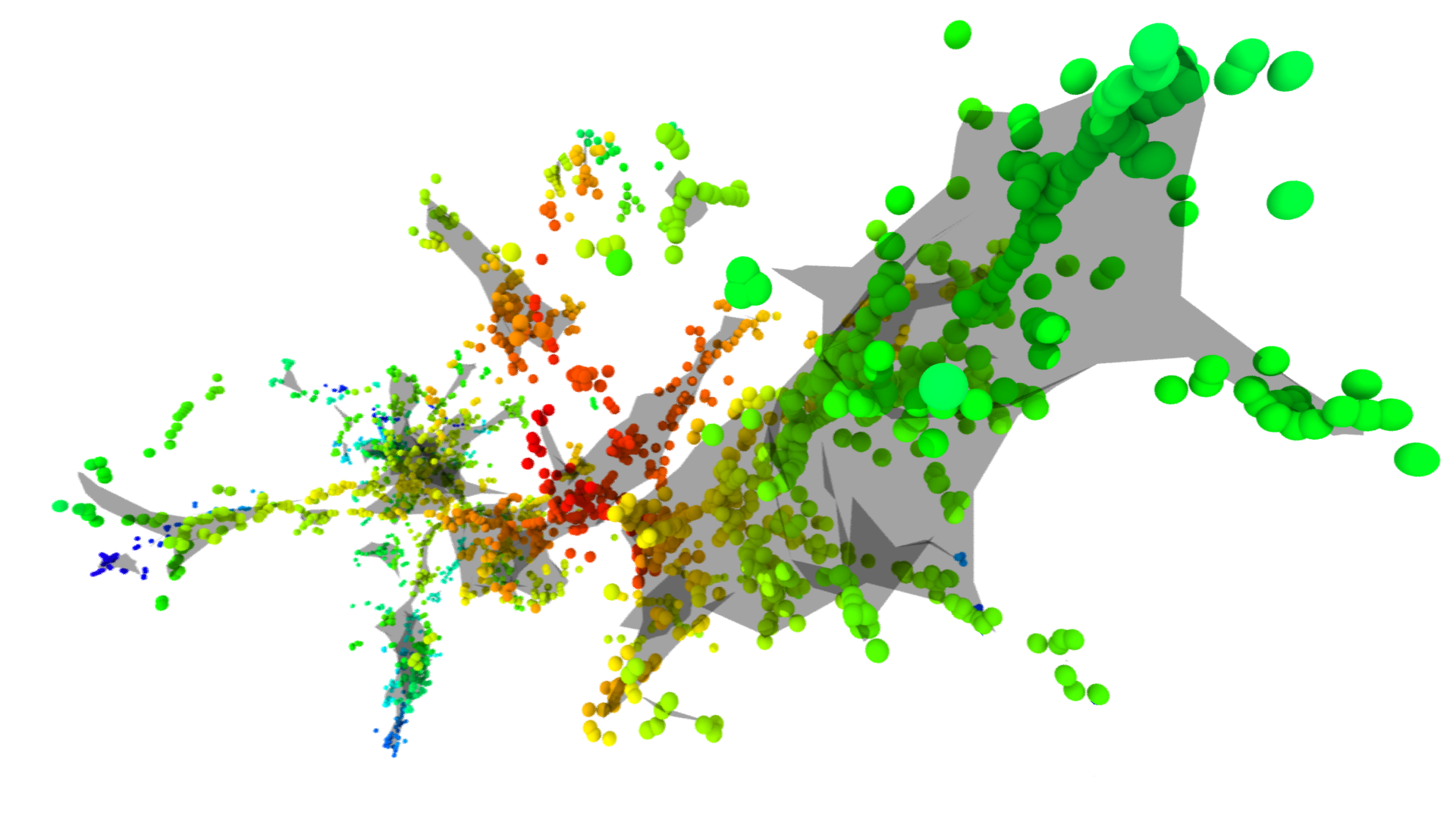
When an energetic ion enters a crystalline solid, the ion can collide with atoms in the lattice which are then displaced and go on to produce additional collisions. This proces continues along the path of the ion create a so-called cascade of defects. Modeling such cascades can reveal unique properties of the ion-solid interaction process such as the cascade density. The effect of cascade density on radiation defect dynamics is studied in detail in the paper “Deterministic Role of Collision Cascade Density in Radiation Defect Dynamics in Si”.
This blog post walks through the method used to determine the cascade density in the paper mentioned above using a combination of the TRansport of Ions in Matter (TRIM) software [1], Open Visualization Tool (OVITO) [2], and python. The cascade densities are calculated using a method similar to that proposed by Heinisch and Singh [3] in which the cascade density is defined as the average local density of vacancies within some averaging radius.
The following outline the steps necessary to calculating the cascade density.
Setting up your environment
TRIM
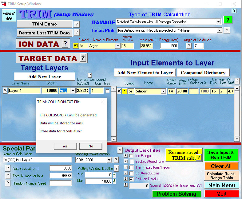
First download SRIM/TRIM software which is freely available here. Once installed, you can open a TRIM simulation, select the ion parameters you wish to use, then select “Detailed Calculation with full Damage Cascade” from the drop down DAMAGE menu, and check the Collision Details box under Outpout Disk Files. The configuration used in this post is shown below.
OVITO
Next, the OVITO library needs to be installed. As mentioned above OVITO is a tool for visual representation of atomic data. However, I’ve found that it has very nice (and efficient) implementations of coordination analysis methods and surface mesh / volume calculation via Delaunay tessellation. The library is installed via:
pip install ovitoImporting TRIM results into python
Now that the environment is setup, we can move towards performing an actual simulation. After running TRIM with the settings specified above, an output file should be created in the SRIM Outputs directory. This file keeps track of the collision events positions, energy, recoil energy, etc., but is not easy to import and use for analysis in its current form. The script below parses the file and output the results as a pandas dataframe:
import sys, os
import numpy as np
import pandas as pd

def parse_trim_file(filename, ion_count=1e9):
    """
    Input::
      filename: filename/path [str]
      ion_count: number of ions [int]
    Output::
      pandas dataframe containing ions 1 to ion_count
    """
    fh = open(filename, 'r', encoding='ISO-8859-1')
    cascades = fh.readlines()
    cascades_df = pd.DataFrame()
    recoil = []
    atom = []
    energy = []
    x = []
    y = []
    z = []
    vac = []
    repl = []
    ion = []
    for line in cascades[26:]:
        data = line.split()
        if data:
            if (data[0] == 'Recoil'):
                ion_number = int(data[-1][:-1])
                if ion_number > ion_count:
                    df = pd.DataFrame({'recoil':recoil, 'atom':atom, 'energy':energy,
                       'x':x, 'y':y, 'z':z, 'vac':vac, 'repl':repl, 'ion':ion})
                    return df
            elif data[0] == chr(219): #chr(219) character at start of every collision entry
                recoil += [int(data[1])]
                atom += [int(data[2])]
                energy += [float(data[3])]
                x += [float(data[4])]
                y += [float(data[5])]
                z += [float(data[6])]
                vac += [int(data[7])]
                repl += [int(data[8])]
                ion += [ion_number]
    df = pd.DataFrame({'recoil':recoil, 'atom':atom, 'energy':energy,
                       'x':x, 'y':y, 'z':z, 'vac':vac, 'repl':repl, 'ion':ion})
    return df
OVITO Simulation Class
In order to make importing new ion cascades easier, the following class has been created to interface with OVITO. The Class is initialized by passing the x,y,z positions of defects along with the yz-plane minimum and maximum dimensions.
import ovito as ov
import numpy as np
import pandas as pd

class OvitoSimulation():
    def __init__(self, xyz=None, yz_plane=None, cell_vec=None):
        """
        Input::
            xyz (numpy array): x,y,z positions of defects of shape (n, 3) where n is the
                number of defects
            yz_plane: ion collisions occur along the x-axis and the yz-plane defines the
                surface over which cascades are incident.
        """
        self.xyz = xyz
        self.yz_plane = yz_plane
        self.cell_vec = cell_vec
        if not xyz is None:
            self.create_node()
        else:
            self.xyz = np.empty(shape=(0,3))
    def create_node(self):
        """
        Create simulation cell
        """
        if self.cell_vec == None:
            cell = ov.data.SimulationCell()
            x_max = np.max(self.xyz[:,0]) + 50
            xyz_max = np.array([x_max, np.abs(self.yz_plane[0,:][1] - self.yz_plane[0,:][0]),
                                np.abs(self.yz_plane[1,:][1] - self.yz_plane[1,:][0])])
            xyz_vec = xyz_max*np.identity(3)
            origin = np.array([[-25,self.yz_plane[0,:].min(),self.yz_plane[0,:].min()]])
            self.cell_vec = np.concatenate([xyz_vec, origin.T], axis=1)
        cell.matrix = self.cell_vec
        cell.pbc = (False, False, False)
        cell.display.line_width = 0.1

        particles = ov.data.Particles()
        particles.create_property("Position", data=self.xyz)
        data = ov.data.DataCollection(objects = [particles])
        data.add(cell)
        self.pipeline = ov.pipeline.Pipeline(source = ov.pipeline.StaticSource(data = data))

    def coordination(self, cutoff = 100.0, bins = 200):
        """
        Counts the number of neighbors for each particle that are within a given cutoff range
        around its position.
        Parameters::
            cutoff (float): cutoff range to look for particles.
            bins (int): number of bins to use when creating the radial distribution function.
        """
        modifier = ov.modifiers.CoordinationNumberModifier(cutoff = cutoff,
            number_of_bins = bins)
        self.pipeline.modifiers.append(modifier)
        modifier = ov.modifiers.HistogramModifier(bin_count=bins,
            particle_property="Coordination")
        self.pipeline.modifiers.append(modifier)
        coord = self.pipeline.compute()
        return coord.series['histogram[Coordination]'].as_table()
Finally, one last function is needed to rearrange the cascades from the TRIM data file as we see fit. For isolated cascade calculations you can set the simulation cell size to be much larger than the area occupied by cascades so that every cascade is essentially isolated. Of course this method can also be used to study the interaction of collision cascades.
def create_pulse(ion_df, yz_plane):
    """
    ion_df = dataframe of ions
    yz_plane = 2d np array containing min/max values (Ang)
    """
    area = (yz_plane[0][0] - yz_plane[0][1])*(yz_plane[1][0] - yz_plane[1][1])
    num_ions = len(ion_df['ion'].unique())
    ion_positions = np.random.rand(2,num_ions).T
    ion_positions = yz_plane.min(axis=1) + np.abs(yz_plane[:,0] - yz_plane[:,1])*ion_positions
    ions = ion_df['ion'].unique()
    pulse = pd.DataFrame()
    for ion, pos in zip(ions,ion_positions):
        ion_array = ion_df[ion_df['ion'] == ion][['x','y','z']].copy()
        ion_array[['y','z']] += pos
        pulse = pd.concat([pulse,ion_array])
    try:
        return pulse[['x','y','z']].values
    except:
        return pulse
An Example
This section goes through an example using 500 keV Ar+ ions incident onto Si. The TRIM file created for this example had ~6000 ion cascades and was ~2.8 GB. The code below parses this file into a pandas dataframe in approximately 2 minutes on my Dell XPS13 laptop.
ion_df = parse_trim_file('./COLLISON_500keV_Ar_Si6000.txt',500)
ion_df_slice = ion_df[(ion_df['x'] < 6000) & (ion_df['x'] > 4000)].reset_index(drop=True)
The depth dependence of vacancies can be plotted as shown below:
plt.hist(ion_df['x'], bins = 50, stacked=True, density=True)
plt.xlabel('Depth (Ang.)')
plt.ylabel('Count')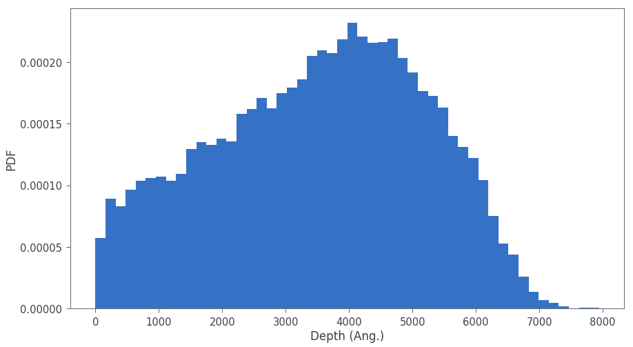
Next we can calculate the local cascade density for each vacancy near the depth of maximum vacancy concentration. The cascade density is returned as a histogram across density values (plotted below in Fig. 4). The average cascade density for the averaging radius of 10 nm is calculated in the last line of the snippet below.
ion_df_slice = ion_df[(ion_df['x'] < 6000) & (ion_df['x'] > 4000)].reset_index(drop=True)
xyz_ions = create_pulse(ion_df_slice, yz_plane)
ions_ov = OvitoSimulation(xyz=xyz_ions, yz_plane = np.array([[-1e6,1e6],[-1e6,1e6]]))
coord = ions_ov.coordination(bins=120) / ((4./3.)*np.pi*10**3)
density = coord.copy()
density[:,0] /= ((4./3.)*np.pi*10**3)

plt.scatter(density[:,0], density[:,1])
plt.xlabel('Density')
plt.ylabel('Count')
plt.show()

print('Average cascade density is: ', np.sum(density[:,0]*density[:,1]/np.sum(density[:,1])))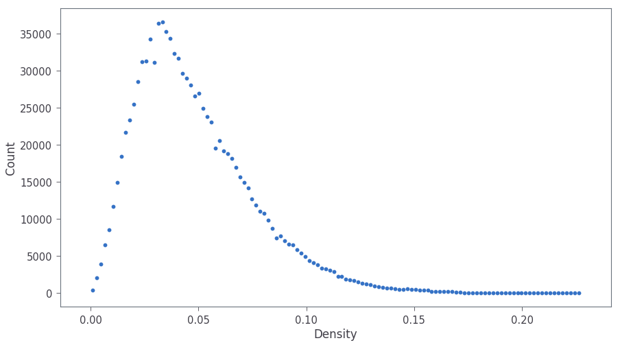
The average cascade density for an averaging radius of 10 nm is calculated in the last line of the snippet above as 0.0481 Vac./nm3.
Resources and Additional Reading
[1] TRIM/SRIM software: http://www.srim.org/SRIM/SRIMLEGL.htm
[2] OVITO software: https://www.ovito.org/
[3] Heinisch, H. L. & Singh, B. N. On the structure of irradiation-induced collision cascades in metals as a function of recoil energy and crystal structure. Phil. Mag. A 67, 407–424 (1993).